Hunting for Cobalt Strike: Mining and plotting for fun and profit

Introduction

Cobalt Strike is a commercial Command and Control framework built by Helpsystems. You can find out more about Cobalt Strike on the MITRE ATT&CK page. But it can also be used by real adversaries. In this post we describe how to use RiskIQ and other Microsoft technologies to see if you have Cobalt Strike payloads (also called “beacons”) in your network.

Hunting for Cobalt Strike beacons across large environments can be a challenge for threat hunting teams. But with that comes a great amount of creativity and opportunity. In this blog post, the Microsoft Security Response Center’s (MSRC) Threat Hunting team seeks to improve the visibility of our environment, for both internal security and our customers, by exploring hunting methodologies for Cobalt Strike Command and Control (C2) traffic.

Finding Cobalt Strike Team Servers

In January 2021, RiskIQ released a blog post discussing the utilization of JARM hashes to identify malicious infrastructure across the internet in their platform. Since then, there’s been an ever-increasing number of threat hunting groups and SOC’s utilizing JARM hashes within their organizations to detect malicious activity. Later that year, at the SANS Threat Hunting Summit & Training 2021, José Hernandez and Michael Haag presented a fantastic framework to the community for utilizing internet scanning services combined with JARM hashes to pull lists of potential Cobalt Strike Team Servers. These IPs are then probed for the beacon config, utilizing an open source NMAP script by Wade Hickey and Zach Stanford. You can find out more about JARM here.

As explained by José Hernandez and Michael Haag in their SANS Threat Hunting Summit talk, there are several benefits to identifying Cobalt Strike servers by utilising scanning services like Microsoft Defender Threat Intelligence. The primary one is that we avoid scanning the entire internet, which can be problematic. We also can leverage the multitude of data types they collect to vary our capabilities in identifying teams’ servers. Three such data types are Jarm Fuzzy Hashing, Banners, and TLS Serials/hashes.

One thing to note about using JARM hashes are that they do not always provide exact answers for finding Cobalt Strike Team Servers. As demonstrated by Raphael Mudge on HelpSystems website, JARM fingerprints can be altered based on the server configuration. Thus, it can be fruitful to utilize other data types within internet scanning datasets.

In our fork of José Hernandez and Michael Haag’s framework, we utilize JARM fuzzy hashing, banners, and TLS Serials/hashes. We have a public example of this implementation with a RiskIQ module for JARM & TLS Hashes here.

Below highlights an example module implementation of the Melting-Cobalt framework utilizing the RiskIQ Community API’s SSL Certificate class to pull all IP addresses that match the SHA1 hash for default Cobalt Strike Team Servers:

‘6ece5ece4192683d2d84e25b0ba7e04f9cb7eb7c’

Figure 1 Example of API calls to RiskIQ to get SSL Certificate hash

We can run this scanner by using a Virtual Machine in Azure, or by utilizing serverless solutions such as Azure Functions. We can then start to pull IP addresses from our scanning service API’s and probe them for Cobalt Strike beacons. If a Cobalt Strike beacon is returned, we store the data ready for ingest into our database.

Figure 2 Example of an extracted Cobalt Strike beacon

Now that we have discussed a methodology to identify Cobalt Strike Team Servers and carve out beacon configs, we need somewhere to ingest the data to begin hunting.

Since we here at Microsoft have a large amount of infrastructure, we like to utilize fast and scalable data analytics platforms to support our hunting such as Microsoft Sentinel and Azure Data Explorer. In a later blog post, we will discuss utilizing Microsoft Sentinel to use this data to hunt within your SIEM environment. To find out more how you can integrate such a feed to your Sentinel instance, head over to Microsoft Docs where you can learn more about ingesting STIX/TAXII feeds to Sentinel. Ingesting the extracted Cobalt Strike beacons to your Sentinel instance, can be a quick and effective way to correlate network data in your SIEM.

But for now, we will discuss how you can utilize this data within Azure Data Explorer. This enables us to have great insights into streaming data, time-series analysis, and an advanced query language to build models to detect patters within our network data. Ingesting and plotting the data

As a hunting team, we love to use Kusto Query Language (KQL) to build hunting queries and produce signals. Azure Data Explorer (in addition to products like Sentinel) provide great hunting grounds based on where your data sits. To ingest data to Azure Data Explorer using Python, we have a simple to use application that can get you started: azure-kusto-python/quick_start at master · Azure/azure-kusto-python (github.com).

An example Kusto configuration for ingesting our Cobalt Strike Beacon data can be found below, where we are ingesting data to a table called “CobaltStrikeActiveDiscovery”:

{
 "kustoUri" : "https://YOURADXCLUSTER.kusto.windows.net",
 "ingestUri" : "https://ingest-YOURADXCLUSTER.kusto.windows.net",
 "databaseName" : "ThreatHunting",
 "tableName" : "CobaltStrikeActiveDiscovery",
 "useExistingTable": false,
 "alterTable": true,
 "queryData": true,
 "ingestData": true,
 "tableSchema" : "(TIMESTAMP:datetime, nmap_cmd:string, ip:string, port:string, protocol:string, service:string, hostnames:string, x64_sha1:string, x64_sha246:string, x64_md5:string, x86_sha1:string, x86_sha256:string, x86_md5:string, x64_config_method_1:string, x64_config_method_2:string, x64_config_port:string, x64_config_spawn_to_x64:string, x64_config_spawn_to_x86:string, x64_config_jitter:string, max_dns:string, dns_idle:string, dns_sleep:string, user_agent:string, watermark:string, c2_host_header:string, x64_config_polling:string, x64_config_c2_server:string, x64_config_beacon_type:string, x64_config_http_method_path_2:string, x64_uri_queried:string, x86_config_method_1:string, x86_config_method_2:string, x86_config_port:string, x86_config_spawn_to_x64:string, x86_config_spawn_to_x86:string, x86_config_jitter:string, x86_config_polling:string, x86_config_c2_server:string, x86_config_beacon_type:string, x86_config_http_method_path_2:string)",
 "data" :
 [
  {
   "sourceType": "localFileSource",
   "dataSourceUri": "results.json",
   "format": "MULTIJSON",
   "useExistingMapping": false,
   "mappingName": "CobaltStrikeMapping",
   "mappingValue": "[{\"Properties\":{\"Path\":\"$.TIMESTAMP\"},\"column\":\"TIMESTAMP\",\"datatype\":\"datetime\"}, {\"Properties\":{\"Path\":\"$.nmap_cmd\"},\"column\":\"nmap_cmd\",\"datatype\":\"string\"}, {\"Properties\":{\"Path\":\"$.ip\"},\"column\":\"ip\",\"datatype\":\"string\"}, {\"Properties\":{\"Path\":\"$.port\"},\"column\":\"port\",\"datatype\":\"string\"}, {\"Properties\":{\"Path\":\"$.protocol\"},\"column\":\"protocol\",\"datatype\":\"string\"}, {\"Properties\":{\"Path\":\"$.service\"},\"column\":\"service\",\"datatype\":\"string\"}, {\"Properties\":{\"Path\":\"$.hostnames\"},\"column\":\"hostnames\",\"datatype\":\"string\"}, {\"Properties\":{\"Path\":\"$.x64_sha1\"},\"column\":\"x64_sha1\",\"datatype\":\"string\"}, {\"Properties\":{\"Path\":\"$.x64_sha246\"},\"column\":\"x64_sha246\",\"datatype\":\"string\"}, {\"Properties\":{\"Path\":\"$.x64_md5\"},\"column\":\"x64_md5\",\"datatype\":\"string\"}, {\"Properties\":{\"Path\":\"$.x86_sha1\"},\"column\":\"x86_sha1\",\"datatype\":\"string\"}, {\"Properties\":{\"Path\":\"$.x86_sha256\"},\"column\":\"x86_sha256\",\"datatype\":\"string\"}, {\"Properties\":{\"Path\":\"$.x86_md5\"},\"column\":\"x86_md5\",\"datatype\":\"string\"}, {\"Properties\":{\"Path\":\"$.x64_config_method_1\"},\"column\":\"x64_config_method_1\",\"datatype\":\"string\"}, {\"Properties\":{\"Path\":\"$.x64_config_method_2\"},\"column\":\"x64_config_method_2\",\"datatype\":\"string\"}, {\"Properties\":{\"Path\":\"$.x64_config_port\"},\"column\":\"x64_config_port\",\"datatype\":\"string\"}, {\"Properties\":{\"Path\":\"$.x64_config_spawn_to_x64\"},\"column\":\"x64_config_spawn_to_x64\",\"datatype\":\"string\"}, {\"Properties\":{\"Path\":\"$.x64_config_spawn_to_x86\"},\"column\":\"x64_config_spawn_to_x86\",\"datatype\":\"string\"},  {\"Properties\":{\"Path\":\"$.x64_config_jitter\"},\"column\":\"x64_config_jitter\",\"datatype\":\"string\"}, {\"Properties\":{\"Path\":\"$.max_dns\"},\"column\":\"max_dns\",\"datatype\":\"string\"}, {\"Properties\":{\"Path\":\"$.dns_idle\"},\"column\":\"dns_idle\",\"datatype\":\"string\"}, {\"Properties\":{\"Path\":\"$.user_agent\"},\"column\":\"user_agent\",\"datatype\":\"string\"}, {\"Properties\":{\"Path\":\"$.watermark\"},\"column\":\"watermark\",\"datatype\":\"string\"},  {\"Properties\":{\"Path\":\"$.c2_host_header\"},\"column\":\"c2_host_header\",\"datatype\":\"string\"}, {\"Properties\":{\"Path\":\"$.x64_config_polling\"},\"column\":\"x64_config_polling\",\"datatype\":\"string\"}, {\"Properties\":{\"Path\":\"$.x64_config_http_method_path_2\"},\"column\":\"x64_config_http_method_path_2\",\"datatype\":\"string\"}, {\"Properties\":{\"Path\":\"$.x64_config_beacon_type\"},\"column\":\"x64_config_beacon_type\",\"datatype\":\"string\"}, {\"Properties\":{\"Path\":\"$.x64_uri_queried\"},\"column\":\"x64_uri_queried\",\"datatype\":\"string\"}, {\"Properties\":{\"Path\":\"$.x86_config_method_1\"},\"column\":\"x86_config_method_1\",\"datatype\":\"string\"}, {\"Properties\":{\"Path\":\"$.x86_config_method_2\"},\"column\":\"x86_config_method_2\",\"datatype\":\"string\"}, {\"Properties\":{\"Path\":\"$.x86_config_port\"},\"column\":\"x86_config_port\",\"datatype\":\"string\"}, {\"Properties\":{\"Path\":\"$.x86_config_spawn_to_x64\"},\"column\":\"x86_config_spawn_to_x64\",\"datatype\":\"string\"}, {\"Properties\":{\"Path\":\"$.x86_config_spawn_to_x86\"},\"column\":\"x86_config_spawn_to_x86\",\"datatype\":\"string\"}, {\"Properties\":{\"Path\":\"$.x86_config_jitter\"},\"column\":\"x86_config_jitter\",\"datatype\":\"string\"}, {\"Properties\":{\"Path\":\"$.x86_config_polling\"},\"column\":\"x86_config_polling\",\"datatype\":\"string\"}, {\"Properties\":{\"Path\":\"$.x86_config_c2_server\"},\"column\":\"x86_config_c2_server\",\"datatype\":\"string\"}, {\"Properties\":{\"Path\":\"$.x86_config_beacon_type\"},\"column\":\"x86_config_beacon_type\",\"datatype\":\"string\"}, {\"Properties\":{\"Path\":\"$.x86_config_http_method_path_2\"},\"column\":\"x86_config_http_method_path_2\",\"datatype\":\"string\"}]"
  }
 ]
}

Once ingested to Kusto, your Azure Data Explorer dataset should look like this:

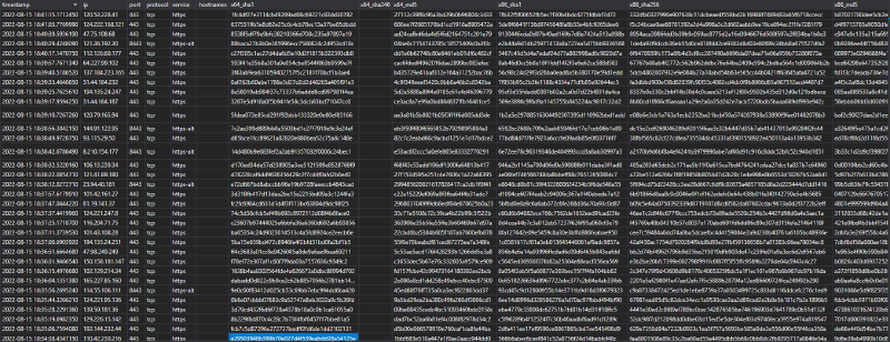
Figure 3 Example of Beacon Data ingested into Azure Data Explorer dataset #1

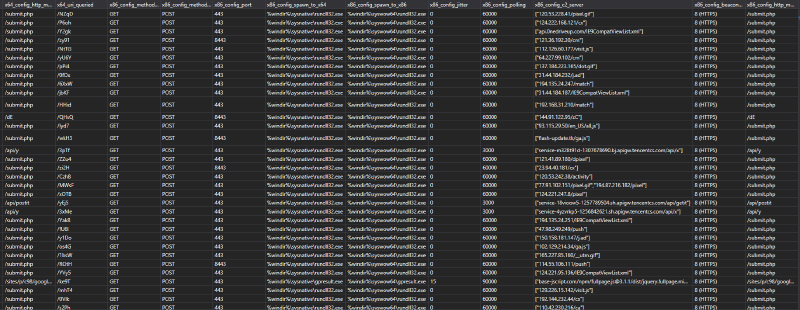
Figure 4 Example of Beacon Data ingested into Azure Data Explorer dataset #2

You can see that we’re able to have valuable data streaming to this database ready for us to build data analytics over the top. Using https://dataexplorer.azure.com/, we can plot some insights aspects of the data in Dashboards that supports threat hunting activity using Kusto Query Language. Here are some examples using the multiple visual types available to us when adding a tile in the Data Explorer dashboard:

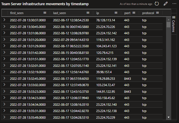
Figure 5 Example table showing Team Server infrastructure movements by timestamp

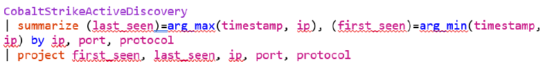
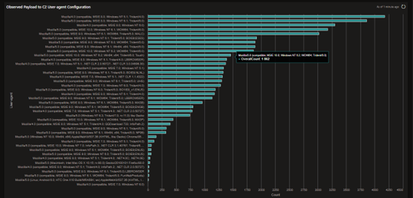
Figure 6 Example bar chart showing count of Payload C2 user-agent configurations

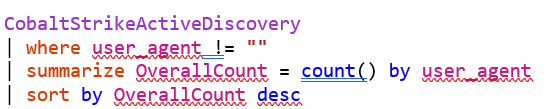
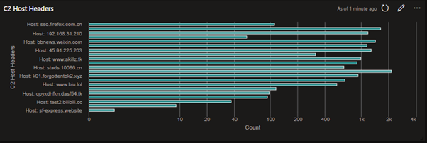
Figure 7 Example bar chart showing C2 Host Headers

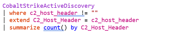
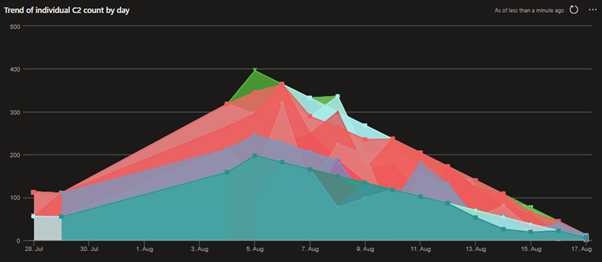
Figure 8 Example area chart showing the Cobalt Strike Team Server volume trend per day

To build more advanced dashboards, we can utilize the multitude of data analytic functions built into Kusto Query Language (KQL). We can start to utilize this data to correlate it against other data sources, such as our internal network data.

Hunting for potential compromises in the network

One great thing about Azure Data Explorer, is that you can bring multiple datasets together and build efficient time series analysis. A key important note is that our data collection pays off by allowing us to get metrics on beacon configurations across the internet to support our hunting. Two key data points to hunt in network data are Polling (or sleep) and Jitter. These are determined by the operator or left as default to set the following configurations:

Polling or Sleep Time: The sleep time between each beacon callback in milliseconds

Jitter: The % of jitter on the polling time. The default is set to 0. A good example of in a configuration we have seen in the below screenshot: If the polling time is set to 25000 milliseconds, which rounds to 25 seconds and a jitter rate is set to 37% (37% of 25 = 9.25), the beacon would sleep between call backs anywhere between 15.75 and 34.25 seconds.

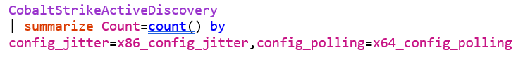
If we look across a sample set of our scanner data, we can gauge a picture of what configurations actors are using. In this snapshot below, we can see that the most common Jitter & Polling configuration is the default one, Jitter set to 0 and Polling rate set to 1 minute.

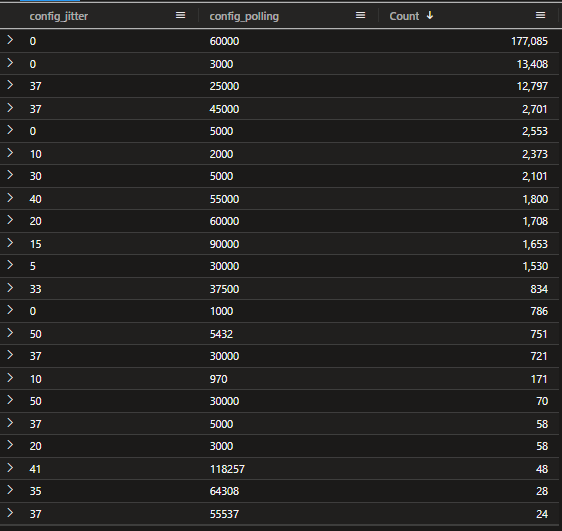
Figure 9 Example snapshot of Jitter and Polling rates

Plotting our Polling configuration, we can see that 80.1% of our data has the default polling rate set to 1 minute. With 30 seconds being the second most common. With an average of 51959 milliseconds or 51.959 seconds.

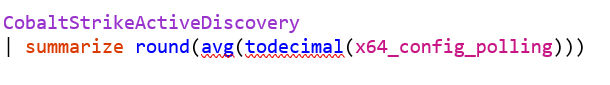
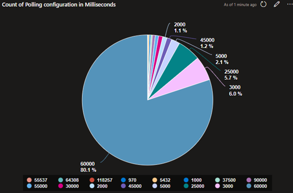
Figure 10 Polling configuration in Milliseconds

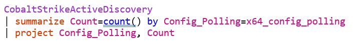
Going further, if we plot our Jitter configurations, seen in figure 11, we can see that 86% of our configurations are set to 0% Jitter. Using the Avg function in Kusto, we calculate the average across the dataset, resulting in an average Jitter percentage of 4%. This should allow us to get a better picture of the variance in frequency across our network data.

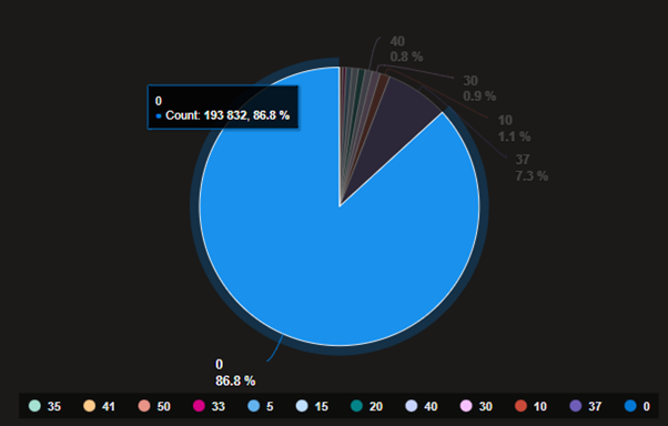
Figure 11 Plotting the jitter configurations

This gives us some interesting insights to look at when correlating our C2 data against our network data. Since the average polling time is 51.95 seconds and the average jitter time is 4%, on average we may see beacon traffic in our data showing callbacks on average between 49.87 seconds and 54.03 seconds. This is of course an average calculation across a sampled data set, but gives us as threat hunters an idea of what we may see when hunting for Cobalt Strike.

To leverage this further, let’s correlate the C2 data we’ve got and correlate it against our network data. You can use a multitude of network data to perform this hunting, whether you capture Zeek or netflow, for example.

Using Azure Logic Apps, we created a daily snapshot of network data that was talking to the C2s captured in our scanner data. We can do this by building Azure Logic App to run on daily cadence, with the Run async control command to ingest a dataset where any of our network traffic has a destination address of a C2 we have in our Cobalt Strike dataset. This should give us a daily feed of all network traffic relating to C2s that we can use to build time-series data.

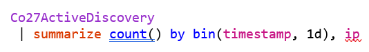
We can use the make-series to create a series of aggregated requests per hour across the last 7 days. This would give us an indication of any beacon traffic that we can observe in this network. Here is an example query:

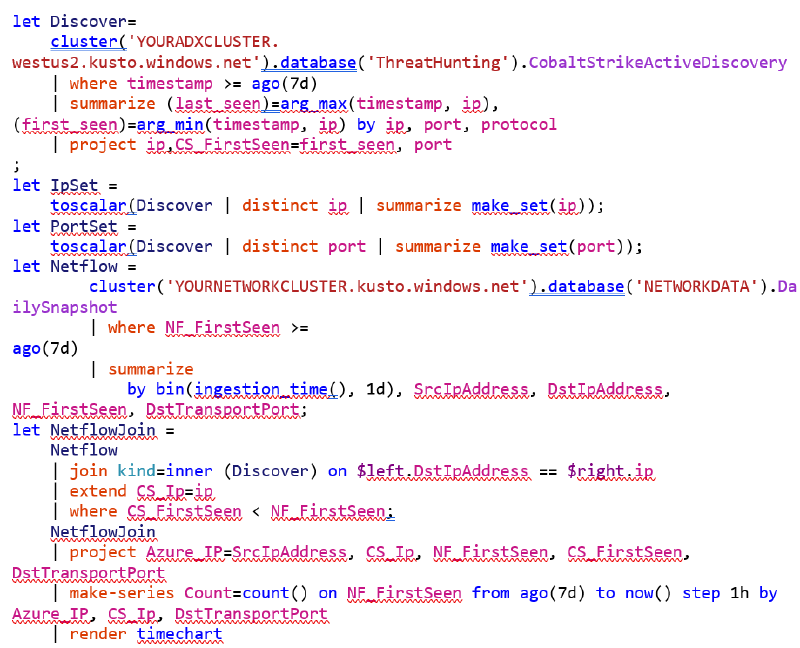
The result may look something like this:

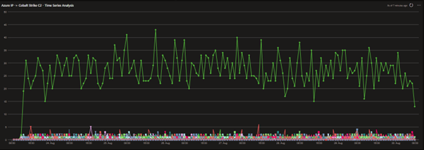
Figure 12 Plotting time series analysis across network data

In our example shown above, we can see an immediate outlier within our data within the plotted green line. We see one machine, talking frequently to a Cobalt Strike C2 from our internal traffic over the last 7 days. This provides us an immediate place to start hunting for compromise, since this machine is talking externally at such a frequent rate it stands out as a predominant anomaly. The data shown above overall shows very small amounts of interactions with our Cobalt Strike C2s per hour. It’s unlikely that they could be compromised machines due to the low volume.

NOTE: In this example, the network data we are using is sampled, which results in the count being lower than a polling rate of ~51.959 seconds.

With full fidelity network data, you may see an average count per hour of around ~50-~70 flows, however this does not encompass additional network data that can be captured during a suspected incident by an attacker interacting with a compromised machine, which will create a higher traffic count. In situations where you see a traffic count higher than the average polling rate, you may then be seeing examples of where the compromised machine is being interacted with by the attacker. This provides even more information about the compromise, including what time the attackers are interacting with the machine which can support time-zone attributions, etc.

In this example, this machine was compromised by Cobalt Strike, and our Time-Series analysis highlighted it effectively. It provided us with an immediate place to start hunting for compromise without the need for any detections on the machine itself.

In addition, picking out areas of high communication can facilitate hunting strategies and narrow down left and right goal posts when hunting across other mediums such as EDR or ETW datasets.

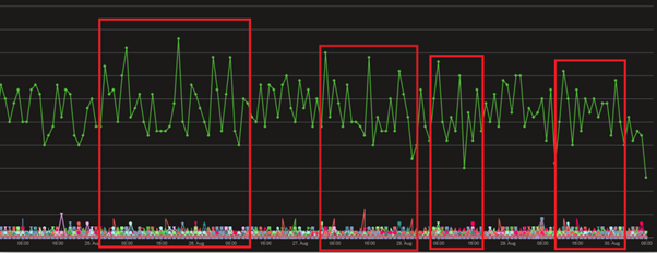
Figure 13 Identifying areas of higher volume network traffic to C2s

Conclusion

As threat hunters, we need to think about multiple ways to identify malicious activity in our environment and cover multiple mediums of data. In this blog post, we’ve discussed an example of utilizing scanning services API data, such as Risk IQ, to identify Cobalt Strike Team Servers, their C2’s and their beacon configuration. We’ve then demonstrated how to utilize this data to build effective ways of gaining valuable insight into what Cobalt Strike might look like in our environment, and ways of utilizing Time-Series analysis to identify compromise.

MSRC Threat Hunting